Slicer estimated time vs actual print time: build a correction factor

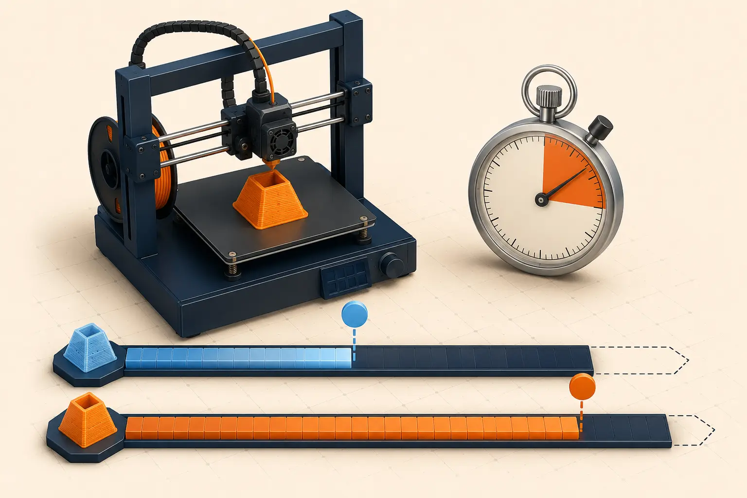
1. Understand what a slicer can predict from the machine profile

The slicer knows the toolpath it generated and the speed, acceleration, jerk or junction, extrusion, cooling, and machine-limit values represented in its profile. When those values match the printer, an estimate can be close. Prusa explicitly notes that its accurate estimates depend on selecting the correct printer profile because machine motion settings differ.

The slicer may not fully represent firmware overrides, a different acceleration limit stored on the printer, user-adjusted speed, bed probing, nozzle cleaning, mesh calibration, heat soak, network transfer, or a manual pause. Identify the boundary shown by the slicer before comparing it with a stopwatch that covers a wider process.

2. Choose consistent start and finish timestamps

For machine-time pricing, start when the printer begins a job and stop when motion ends. For delivery planning, you may need the longer elapsed cycle from file release through warm-up, print, cooldown, removal, and inspection. Both are useful, but mixing them produces a correction factor that cannot explain anything.

Record slicer estimate, machine start, first extrusion if available, print completion, removal-ready time, and direct operator minutes. A camera, printer history, automation log, or simple written timestamps can supply evidence. Use one definition across the comparison set and note power failures, pauses, or interventions as exceptions.

• Save slicer version, printer profile, and generated estimate.
• Define whether actual time includes heating, probing, and cooldown.
• Record overrides, pauses, filament changes, and recovery events.
• Keep operator labor separate from unattended elapsed time.

3. Calculate both the absolute error and the correction ratio

Minutes of error show the schedule impact, while the ratio shows whether the estimate scales. If a four-hour estimate takes four hours twenty minutes, the ratio is about 1.083. Multiplying future estimates from the same validated profile by 1.083 provides a documented planning value until more records are available.

Do not average ratios across unrelated printers, materials, or profiles. A fixed ten-minute probing and warm-up overhead affects a short job much more than a long one, while motion-limit mismatch grows with the toolpath. Maintain a small-job and long-job model if the data shows a consistent fixed component.

4. Use the shape of the error to find the cause

A nearly fixed delay on every job points toward heating, homing, probing, cleaning, or cooldown. A percentage gap that grows with duration suggests mismatched motion limits or speed overrides. Large errors only on small layers may involve minimum layer time and cooling, while multimaterial jobs can add tool-change routines and purging not represented as expected.

Compare the profile with actual firmware limits before applying a permanent pricing buffer. Correcting the source improves completion forecasts and capacity planning. Keep the ratio as a business safeguard, not as a reason to leave a known configuration error unresolved.

5. Use a rolling set of representative completed jobs

Begin with at least ten completed jobs distributed across the durations and materials you sell. Use the median ratio to reduce the influence of one abnormal pause, then inspect the slowest cases separately. Averages are useful for financial planning; the upper end of normal performance is more useful for a delivery promise.

Rebuild the baseline after firmware, slicer, printer profile, nozzle, acceleration, or workflow changes. Preserve the old group rather than silently mixing it with the new one. A versioned correction factor turns a vague complaint that the slicer is wrong into a traceable production metric.

6. Use corrected machine hours for cost, capacity, and promises

Machine depreciation, maintenance reserve, and much of electricity scale with actual machine hours. Multiply the corrected duration by those hourly rates. Direct labor still uses measured hands-on minutes, so a ten-hour unattended print does not automatically become ten hours of labor.

For delivery, add queue time, post-processing, inspection, packing, and a failure-recovery buffer. Corrected printing time is one part of lead time, not the customer's whole promise. The record should make each layer visible so a faster printer, better profile, or simpler workflow produces a measurable benefit.